【seaborn】グラフの作成方法と主な使い方【まとめ】
当ページのリンクには広告が含まれています。

グラフ作成には「matplotlib」と「seaborn」の二つがありますが、よく混合してしまうのでseabornについてまとめてみました。
忘れたときに見に行く場所として記録していきます。
関連記事


【matplotlib】データフレームのグラフ作成方法と主な種類
matplotlibにはx軸・y軸に値を渡してやる方法もありますが、今回はpandasのデータフレームからグラフ生成の方法をご紹介します。 この記事で分かること データフレーム…
関連記事

【matplotlib】グラフの装飾やスタイルの変更方法【まとめ】
matplotlibを使っていると、細かい関数をよく忘れませんか?私はよく忘れてしまいそのたびに調べてしまうので、グラフで使う基本操作をまとめてみました。 この記事で分…
目次
ライブラリのインポート
お決まりのライブラリのインポートです。
import matplotlib.pyplot as plt
import seaborn as sns
import japanize_matplotlib
sns.set(font="IPAexGothic")
%matplotlib inlinejapanize_matplotlibとsns.set(font="IPAexGothic")は日本語フォントを扱う際に文字化け防止用として記入しています。
スタイルの設定
seabornにはset_style("スタイル名")と見た目を変えることができます。
例えば、デフォルトでは
こんな感じで、sns.set("whitegrid")のようにすると
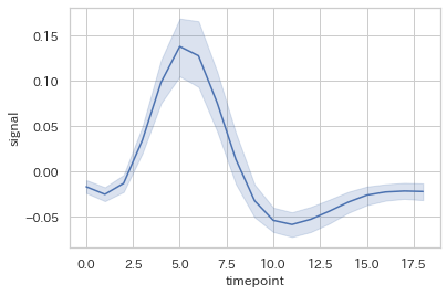
このようにデザインが変化します。
スタイル一覧
| スタイル名 | 背景 | グリッド線 |
|---|---|---|
| darkgrid(デフォルト) | 暗 | あり |
| whitegrid | 白 | あり |
| dark | 暗 | なし |
| white | 白 | なし |
| ticks | 白 | なし, 軸に刻み線あり |
折れ線グラフ
| 引数 | 説明 |
|---|---|
| x, y(省略可) | データフレームのカラム名 |
| data | データフレーム |
| hue | カラムのカテゴリを異なる色で描画 |
| style | カラムのカテゴリを異なる線種で描画 |
| ci | 信頼区間の幅(デフォルト=95)で半透明のエラーバンドを表示 表示しない場合はNone |
| ax | グラフを描画したい領域(axesオブジェクトでの指定) |
まずはデータの準備をします。
seabornに用意されているデータからロードしてグラフを作成してみます。
fmri = sns.load_dataset('fmri')
fmri.head()| subject | timepoint | event | region | signal | |
|---|---|---|---|---|---|
| 0 | s13 | 18 | stim | parietal | -0.017552 |
| 1 | s5 | 14 | stim | parietal | -0.080883 |
| 2 | s12 | 18 | stim | parietal | -0.081033 |
| 3 | s11 | 18 | stim | parietal | -0.046134 |
| 4 | s10 | 18 | stim | parietal | -0.037970 |
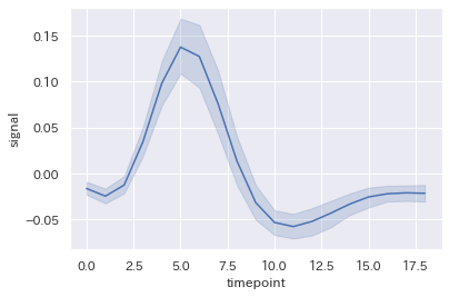
基本形
sns.lineplot(x="timepoint", y="signal", data=fmri)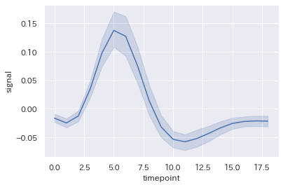
信頼区間の非表示
引数:ci=Noneにて信頼区間を非表示に出来ます。
sns.lineplot(x="timepoint", y="signal", data=fmri, ci=None)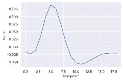
カテゴリ分類
sns.lineplot(x="timepoint", y="signal", data=fmri, hue="region")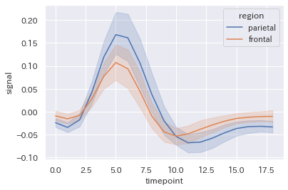
引数:hue="region"でカテゴリ分類がされました。
色も分けられていていい感じですね。
sns.lineplot(x="timepoint", y="signal", data=fmri, hue="region", style="event")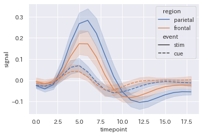
hue, styleは同時に使えます。
自走できるAI人材になるための6ヶ月長期コース【キカガク】
(日本ディープラーニング協会)E資格認定講座!
これまでの受講者数30,000人以上! ・AI人材となり市場価値を高めたい方へ!
棒グラフ
| 引数 | 説明 |
|---|---|
| x, y(省略可) | データフレームのカラム名(xに数値型の変数、yにカテゴリ変数を指定した場合は横棒グラフを描画) |
| data | データフレーム |
| order | 表示する並び(リストで指定) |
| hue | カラムのカテゴリを異なる色で描画 |
| ci | 信頼区間の幅(デフォルト=95)で半透明のエラーバンドを表示 表示しない場合はNone |
| ax | グラフを描画したい領域(axesオブジェクトでの指定) |
下記データを準備しました。
tips = sns.load_dataset('tips')
tips.head()| total_bill | tip | sex | smoker | day | time | size | |
|---|---|---|---|---|---|---|---|
| 0 | 16.99 | 1.01 | Female | No | Sun | Dinner | 2 |
| 1 | 10.34 | 1.66 | Male | No | Sun | Dinner | 3 |
| 2 | 21.01 | 3.50 | Male | No | Sun | Dinner | 3 |
| 3 | 23.68 | 3.31 | Male | No | Sun | Dinner | 2 |
| 4 | 24.59 | 3.61 | Female | No | Sun | Dinner | 4 |
基本形
sns.barplot(x="day", y="total_bill", data=tips)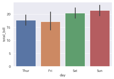
横棒グラフ
y軸にカテゴリ変数を指定した場合には、横棒グラフになります。
sns.barplot(x="tip", y="day", data=tips)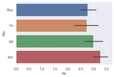
並び順と信頼区間の非表示
カテゴリの並び順はorder=[]とリストで指定し
信頼区間はci=Noneとします。
sns.barplot(x="total_bill", y="sex", data=tips, order=["Male","Female"], ci=None)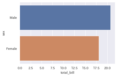
カテゴリ分類
折れ線グラフと同様にhue=""でカラムを指定します。
sns.barplot(x="day", y="total_bill", hue="sex", data=tips)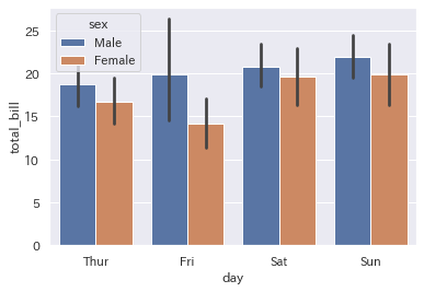
散布図
x, yの指定は必須です。
| 引数 | 説明 |
|---|---|
| x, y | データフレームのカラム名 |
| data | データフレーム |
| hue | カラムのカテゴリを異なる色で描画 |
| style | カラムのカテゴリを異なる線種で描画 |
| size | カラムのカテゴリを異なるサイズで描画 |
| alpha | 透明度 |
| ax | グラフを描画したい領域(axesオブジェクトでの指定) |
データの準備をします。
iris = sns.load_dataset('iris')
iris.head()| sepal_length | sepal_width | petal_length | petal_width | species | |
|---|---|---|---|---|---|
| 0 | 5.1 | 3.5 | 1.4 | 0.2 | setosa |
| 1 | 4.9 | 3.0 | 1.4 | 0.2 | setosa |
| 2 | 4.7 | 3.2 | 1.3 | 0.2 | setosa |
| 3 | 4.6 | 3.1 | 1.5 | 0.2 | setosa |
| 4 | 5.0 | 3.6 | 1.4 | 0.2 | setosa |
基本形
sns.scatterplot(x="sepal_length", y="sepal_width", data=iris)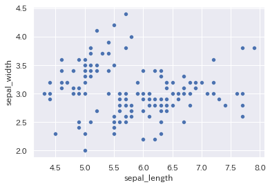
x軸、y軸ともに数値データとなるため、引数:x,yの指定は必須です。
カテゴリ分類
hue—色
sns.scatterplot(x="sepal_length", y="sepal_width", data=iris, hue="species")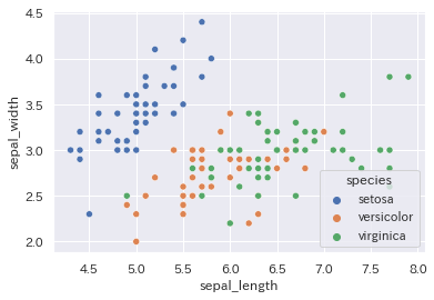
style—マーカー
sns.scatterplot(x="sepal_length", y="sepal_width", data=iris, style="species")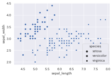
size—大きさ
sns.scatterplot(x="sepal_length", y="sepal_width", data=iris, size="species")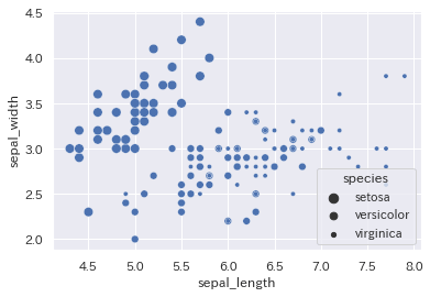
hue, sizeまとめて
sns.scatterplot(x="sepal_length", y="sepal_width", data=iris, hue="species", size="sepal_length")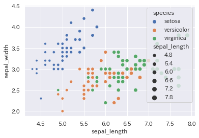
散布図行列
| 引数 | 説明 |
|---|---|
| data | データフレーム |
| hue | カラムのカテゴリを異なる色で描画 |
| kind | 描画するグラフの種類 :scatter・reg |
| diag_kind | 対角線上に描画するグラフの種類 :hist・kde |
基本形
sns.pairplot(data=iris)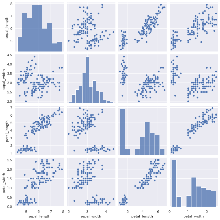
カテゴリ分類
sns.pairplot(data=iris, hue="species")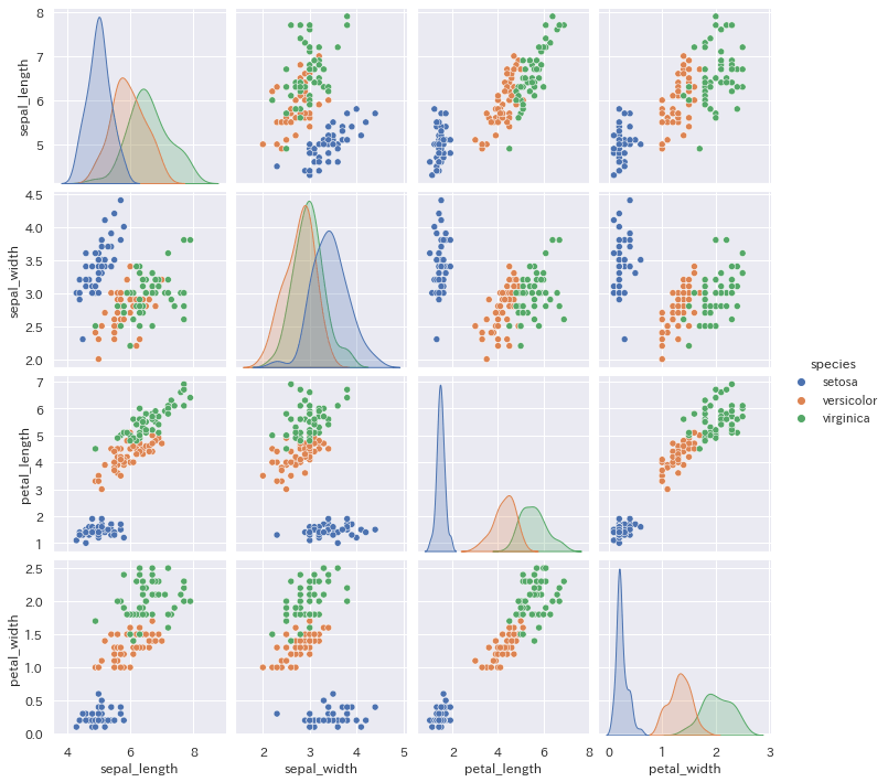
描写するグラフの変更
sns.pairplot(data=iris, hue="species", kind="reg")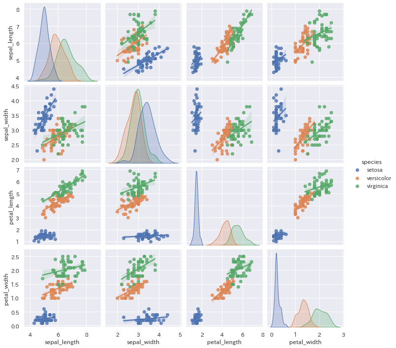
対角線グラフの種類の変更
sns.pairplot(data=iris, hue="species", diag_kind="hist")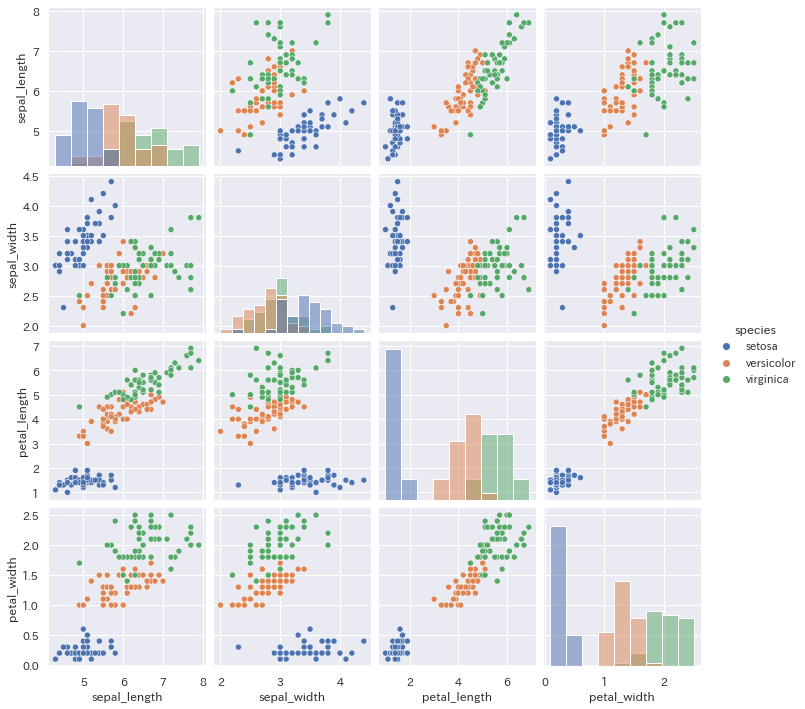
箱ひげ図
| 引数 | 説明 |
|---|---|
| x, y(省略可) | 描画対象のデータのカラム名 |
| data | 描画対象のデータフレーム |
| order | 出力する順番(文字列のリストで指定) |
| hue | 指定したカラムのカテゴリでデータを分割し、グラフを描画 |
| ax | グラフを描画したい領域(axesオブジェクトでの指定) |
基本形
sns.boxplot(x="day", y="total_bill", data=tips)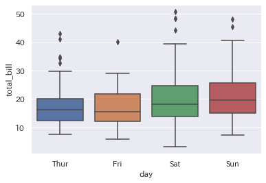
カテゴリ分類
sns.boxplot(x="day", y="total_bill", data=tips, hue="sex")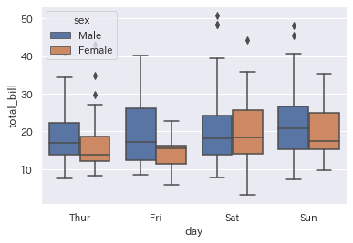
ヒストグラム
| 引数 | 説明 |
|---|---|
| x, y(省略可) | 描画対象のデータのカラム名 |
| data | 描画対象のデータフレーム |
| bin | ビンの分割 |
| stat | 各ビンで計算する統計法 ・count ・frequency ・density ・probability |
| order | 出力する順番(文字列のリストで指定) |
| hue | 指定したカラムのカテゴリでデータを分割し、グラフを描画 |
| ax | グラフを描画したい領域(axesオブジェクトでの指定) |
基本形
sns.histplot(iris["sepal_width"])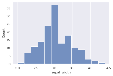
ビンの指定
sns.histplot(iris["sepal_width"], bins=20)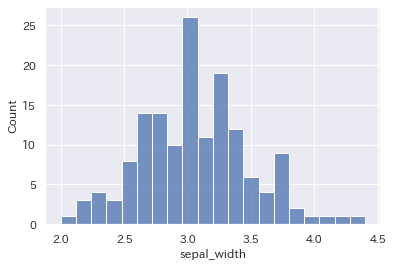
カテゴリ分類
sns.histplot(iris, x="sepal_width", hue="species")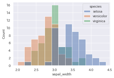
積上げヒストグラム
sns.histplot(iris, x="sepal_width", hue="species", multiple="stack")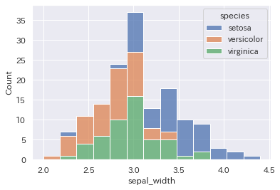
カーネル密度推定の表示
sns.histplot(iris, x="sepal_width", hue="species", kde=True)
自走できるAI人材になるための6ヶ月長期コース【キカガク】
(日本ディープラーニング協会)E資格認定講座!
これまでの受講者数30,000人以上! ・AI人材となり市場価値を高めたい方へ!
ヒートマップ
| 引数 | 説明 |
|---|---|
| x, y(省略可) | 描画対象のデータのカラム名 |
| data | データフレーム |
| bin | ビンの分割 |
| annot | 数値の表示 |
| linewidths | 各セルを分割する線の幅 |
| ax | グラフを描画したい領域(axesオブジェクトでの指定) |
データの準備をします。
flights = sns.load_dataset('flights')
flights.head()| year | month | passengers | |
|---|---|---|---|
| 0 | 1949 | Jan | 112 |
| 1 | 1949 | Feb | 118 |
| 2 | 1949 | Mar | 132 |
| 3 | 1949 | Apr | 129 |
| 4 | 1949 | May | 121 |
ヒートマップ作成のため、ピボットテーブルを作成します。
あわせて読みたい

【pandas】ピボットテーブルの使い方【pivot・pivot_table】
Excelなどでよく使われるピボットテーブル。それをpandasのデータフレームで使う場合には DataFrame.pivot()DataFrame.pivot_table() の2種類があります。今回はピボッ…
flights = flights.pivot("month", "year", "passengers")
flights| year | 1949 | 1950 | 1951 | 1952 | 1953 | 1954 | 1955 | 1956 | 1957 | 1958 | 1959 | 1960 |
|---|---|---|---|---|---|---|---|---|---|---|---|---|
| month | ||||||||||||
| Jan | 112 | 115 | 145 | 171 | 196 | 204 | 242 | 284 | 315 | 340 | 360 | 417 |
| Feb | 118 | 126 | 150 | 180 | 196 | 188 | 233 | 277 | 301 | 318 | 342 | 391 |
| Mar | 132 | 141 | 178 | 193 | 236 | 235 | 267 | 317 | 356 | 362 | 406 | 419 |
| Apr | 129 | 135 | 163 | 181 | 235 | 227 | 269 | 313 | 348 | 348 | 396 | 461 |
| May | 121 | 125 | 172 | 183 | 229 | 234 | 270 | 318 | 355 | 363 | 420 | 472 |
| Jun | 135 | 149 | 178 | 218 | 243 | 264 | 315 | 374 | 422 | 435 | 472 | 535 |
| Jul | 148 | 170 | 199 | 230 | 264 | 302 | 364 | 413 | 465 | 491 | 548 | 622 |
| Aug | 148 | 170 | 199 | 242 | 272 | 293 | 347 | 405 | 467 | 505 | 559 | 606 |
| Sep | 136 | 158 | 184 | 209 | 237 | 259 | 312 | 355 | 404 | 404 | 463 | 508 |
| Oct | 119 | 133 | 162 | 191 | 211 | 229 | 274 | 306 | 347 | 359 | 407 | 461 |
| Nov | 104 | 114 | 146 | 172 | 180 | 203 | 237 | 271 | 305 | 310 | 362 | 390 |
| Dec | 118 | 140 | 166 | 194 | 201 | 229 | 278 | 306 | 336 | 337 | 405 | 432 |
出来ました。
基本形
sns.heatmap(flights)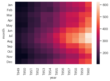
数値の表示
sns.heatmap(flights, annot=True, fmt="d")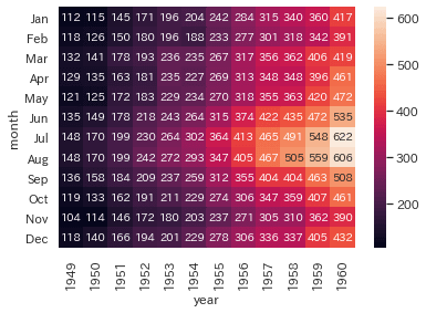
間隔の調整
sns.heatmap(flights, linewidths=1)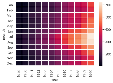
相関変数の可視化
数値間の大小だけではなく、相関関係を確認する場合にも有効です。
値が1に近ければ近いほど、相関が強いということです。
関連記事

変数間の相関関係の確認と可視化方法【pandas・seaborn】
データ分析を行う際に、「説明変数」との関係性を確認する方法として変数間の相関関係を確認する方法があります。 相関関係とは、一方の値が変化した時にもう一方の値も…
sns.heatmap(iris.corr(), annot=True, linewidths=2)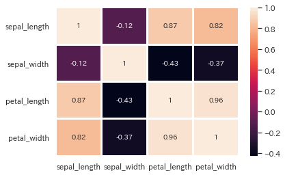
機械学習・データ処理を学ぶのにおすすめの教材
じっくり書籍で学習するなら!


¥2,090 (2022/02/20 08:45時点 | Amazon調べ)
コメント